This blog post is part of our series on potential Bachelor’s and Master’s theses. If you want us to supervise your thesis, contact us. If you just stumbled upon this blog post and want to conduct this project independently of us, please be so kind as to cite this blog post if you ever publish a thesis or research paper based on our proposal.
Summary
This thesis is about implementing and critically analyzing a realistic recommender-system evaluation pipeline. You will run several recommender algorithms on several datasets, vary hyperparameters, random seeds, train-test splits, and possibly other experimental settings, and then analyze whether the resulting evaluation scores can actually be trusted. You will learn how recommender algorithms are evaluated, how metrics such as NDCG, Precision, and Recall are computed, and why a single score can be misleading.
The scientific problem is that recommender-system research often reports only a few final numbers, such as the best NDCG or Precision score. However, these numbers may hide substantial uncertainty. An algorithm may look better only because it was tuned more extensively, tested on a favorable split, evaluated with a lucky random seed, or reported using its best configuration. The thesis therefore asks: how stable are recommender-system evaluation results, which experimental factors influence them most, and when is a reported improvement actually reliable?
The project is similar to a real company scenario: before deploying a recommender system, engineers must compare algorithms, tune hyperparameters, test robustness, and decide which model is reliable enough to use. Since many experiments may be needed, the work will likely involve running jobs on the University of Siegen cluster.
The thesis combines implementation with critical analysis. You will build or adapt an experimental pipeline, but the main goal is not just to produce benchmark tables. The goal is to analyze result distributions, compare stability across algorithms and datasets, identify fragile evaluation conclusions, and develop recommendations for how recommender-system results should be reported. Depending on the focus, the thesis may also investigate whether stable metric values actually correspond to stable recommendation lists for users.
A strong thesis should produce both practical and scientific outcomes: a working experimental setup, a systematic empirical analysis, stability-aware evaluation results, and clear conclusions about when recommender-system comparisons can or cannot be trusted. This could have clear practical value, lead to a publishable research paper, and provide a possible starting point for a PhD or industry career in recommender systems, machine-learning evaluation, reproducibility, or robust model selection.
1. Motivation
Recommender systems are commonly evaluated with metrics such as NDCG@k, Precision@k, Recall@k, MAP, or MRR. These metrics are useful and should not be replaced. However, the way they are commonly reported is often too narrow.
A typical research paper may report a table like this:
| Algorithm | NDCG@10 |
|---|---|
| Algorithm A | 0.800 |
| Algorithm B | 0.810 |
At first glance, Algorithm B seems better. However, this conclusion may be premature. The table hides at least two important questions.
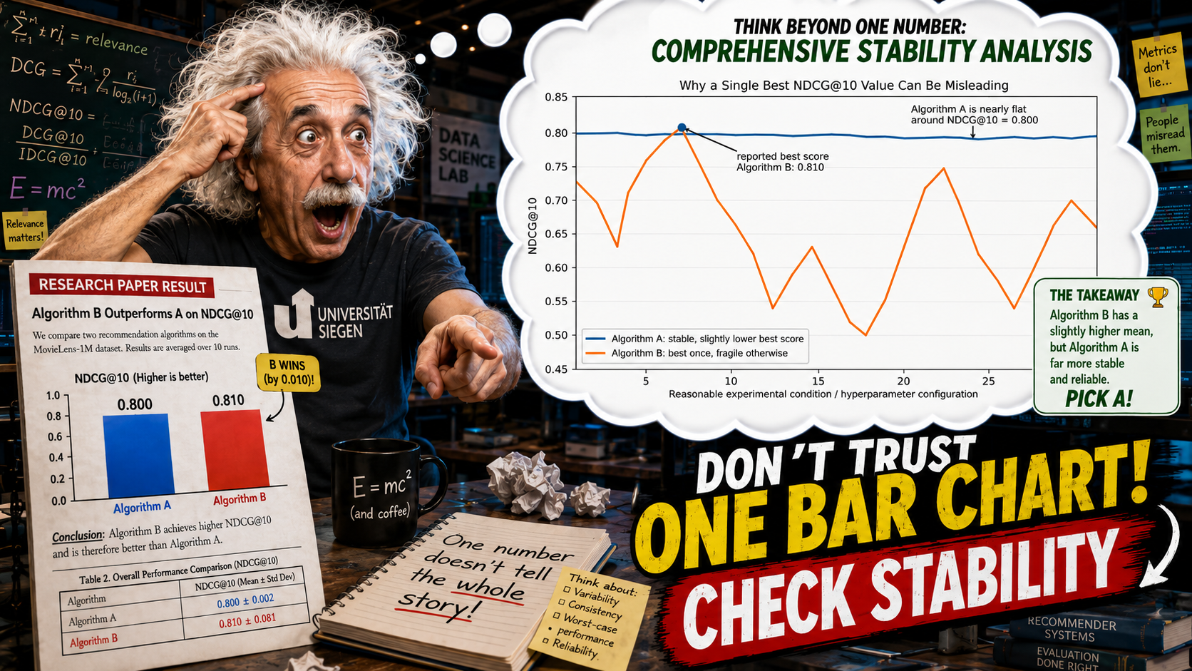
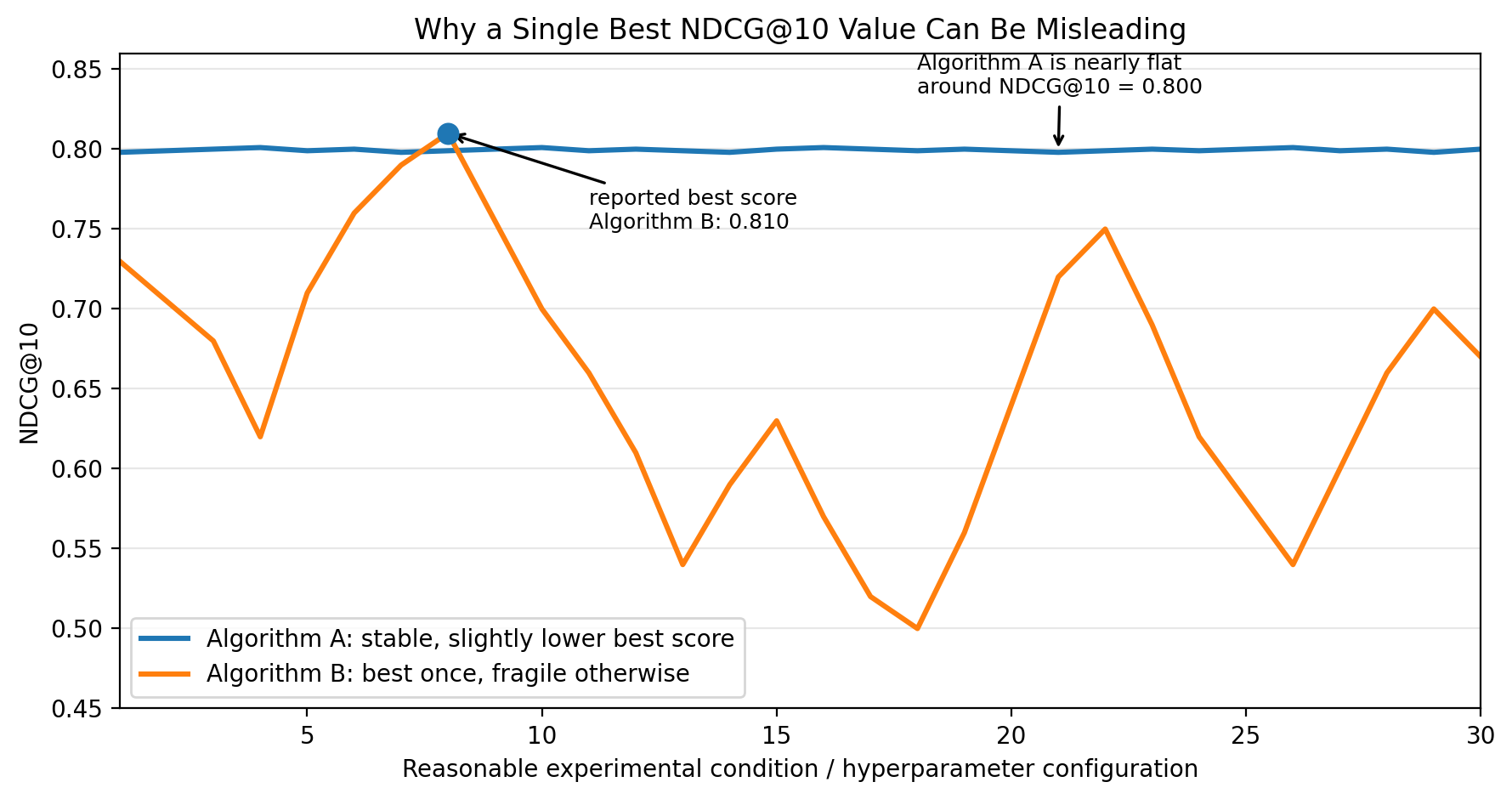
First, how reliable are these metric values? The figure below illustrates why the table alone can be misleading. Algorithm B achieves the highest observed NDCG@10 value, 0.810, in only one experimental condition. This single value could therefore be reported as the “best” result. However, across the remaining reasonable hyperparameter configurations, random seeds, data splits, or datasets, Algorithm B performs substantially worse than Algorithm A. Algorithm A never reaches the same peak value, but its NDCG@10 remains close to 0.800 across almost all conditions. The practical conclusion is that Algorithm B has the better best-case result, while Algorithm A has the more reliable performance profile. For deployment, Algorithm A may therefore be preferable, because its behavior is more predictable and less dependent on finding one favorable configuration.
Second, do similar metric values imply similar recommendations? Two runs of the same algorithm, or two different algorithms from the table above, may both achieve NDCG@10 around 0.800, while recommending largely different items to the same users. Users do not experience NDCG. They experience the recommended items. Therefore, stable or similar metric values do not necessarily imply stable or similar recommendation behavior. This difference can also be practically useful. If Algorithm A and Algorithm B achieve almost the same NDCG but recommend very different relevant items, then neither algorithm may be clearly “better” on its own. Instead, a hybrid or ensemble recommender may be preferable. For example, the system could construct a Top-\(k\) recommendation list by taking the top \(k/2\) recommendations from Algorithm A and the top \(k/2\) recommendations from Algorithm B. In such a case, output differences are not merely a problem for evaluation; they may reveal complementarity between algorithms.
You could therefore investigate one of two closely related forms of stability:
- Metric Stability
How stable are evaluation scores such as NDCG, Precision, and Recall under reasonable experimental variation? - Output Stability
How stable are the actual recommended items under reasonable experimental variation, even when metric values remain similar?
Both directions address the same broader problem: current recommender-system evaluation practice often reports too little information. A single best NDCG value does not tell us how robust, representative, or practically reliable an algorithm is.
The topic is conceptually inspired by earlier work on stability evaluation in event detection. In that work, small changes such as time-window size, stopword handling, and retweet handling substantially influenced the detected events. The underlying idea is directly relevant here: if small experimental choices can change the outcome, evaluation should report more than one best result.
2. Practical Example: Which Algorithm Would You Deploy?
Suppose you have to choose one recommender algorithm for a new system.
| Algorithm | Reported NDCG@10 |
|---|---|
| Algorithm A | 0.800 |
| Algorithm B | 0.810 |
If this is all you know, Algorithm B appears slightly better. But now suppose you evaluate both algorithms under several reasonable hyperparameter settings, random seeds, and data splits.
| Algorithm | Best NDCG@10 | Median NDCG@10 | 10th Percentile | Worst Observed NDCG@10 |
|---|---|---|---|---|
| Algorithm A | 0.805 | 0.798 | 0.790 | 0.785 |
| Algorithm B | 0.810 | 0.710 | 0.540 | 0.410 |
Algorithm B has the best single score. Algorithm A has the more reliable performance distribution.
If the system will be deployed in a real application, with constantly changing data, users etc, then Algorithm A may be preferable. The difference between 0.800 and 0.810 is small, but the difference in reliability is large. Algorithm B may require careful tuning, may be fragile under data changes, and may behave unpredictably when moved to a new environment.
Now consider the same situation from the perspective of output stability.
| Run | NDCG@5 | Recommended Items |
|---|---|---|
| Algorithm A, Run 1 | 0.800 | Dune, Arrival, Blade Runner, Interstellar, The Martian |
| Algorithm A, Run 2 | 0.798 | Dune, Arrival, Blade Runner, Interstellar, Gravity |
| Algorithm B, Run 1 | 0.810 | Dune, Arrival, Blade Runner, Interstellar, The Martian |
| Algorithm B, Run 2 | 0.808 | Her, Ex Machina, Moon, Annihilation, Children of Men |
Algorithm B may appear metric-stable, because its NDCG values are similar. But it may be output-unstable, because the actual recommendations change substantially. This matters when a system should behave predictably, when explanations are required, when user trust matters, or when developers want to understand what the algorithm actually does.
The practical implication is:
A slightly lower but stable algorithm may be better than a slightly higher but unstable algorithm.
However, this statement needs scientific clarification. Stability is not automatically good. A popularity recommender may be extremely stable because it always recommends the same popular items but popularity has other downsides. The research problem is therefore not simply to reward stability. The research problem is to define when stability is useful, how it should be measured, and how it should be reported alongside classical accuracy metrics.
3. Why Current Evaluation Practice Is Insufficient
Current recommender-system evaluation often treats performance as if each algorithm had one true value on each dataset. In practice, performance is a distribution.
A reported NDCG value depends on many choices:
- hyperparameter search space;
- number of tried hyperparameter configurations;
- train/test split;
- validation protocol;
- random seed;
- negative sampling strategy;
- preprocessing choices;
- dataset characteristics;
- evaluation cutoff \(k\);
- candidate item set.
A paper that reports only the best score hides the distribution behind that score. This creates several problems.
3.1 Best-Score Reporting Can Be Misleading
If an algorithm has one excellent configuration and many weak configurations, reporting only the best result overstates its reliability. The result may be real, but not representative.
3.2 Similar Mean Performance Can Hide Different Risk
Two algorithms may have the same average NDCG, but one may be tightly concentrated around the mean while the other has frequent failures.
3.3 Standard Deviation May Be Insufficient
If performance values are normally distributed, mean and standard deviation may be reasonable summaries. But recommender results may be skewed, heavy-tailed, or multimodal.
For example, an algorithm may have two regimes:
- good configurations around NDCG@10 = 0.800;
- failed configurations around NDCG@10 = 0.500.
The mean may be 0.650, but that number describes neither regime well.
3.4 Stable Metrics May Hide Unstable Outputs
Two runs may achieve similar NDCG but recommend different items. This is a deeper problem. It means that the metric value alone is not enough to describe the algorithm’s behavior.
3.5 Scientific Conclusions May Depend on Experimental Choices
A small NDCG difference, such as 0.800 vs. 0.810, may not justify claiming that one algorithm is better if the ranking changes under different splits, seeds, or hyperparameters. Stability-aware evaluation can reveal whether a conclusion is robust or fragile.
4. Two Thesis Directions
Direction A: Metric Stability
Core Question
Instead of asking the trivial question “Do metrics change when the setup changes?”, the more relevant question is:
How much do metric values vary under reasonable experimental variation, which factors cause this variation, and when is the variation large enough to change scientific or practical conclusions?
This direction focuses on NDCG, Precision, Recall, MAP, MRR, or similar metrics.
Example Research Questions
- How large is the variation in NDCG@10 across hyperparameter configurations?
- How much of the variation is caused by hyperparameters, data splits, random seeds, or datasets?
- Are some algorithms high-performing but fragile?
- Are some algorithms slightly weaker but much more reliable?
- Do algorithm rankings change when using robust performance instead of best performance?
- What is the distributional shape of metric values?
- Which stability metrics are most informative for future papers?
Example Hypotheses
- H1: Best-score reporting overestimates the reliability of some recommender algorithms.
- H2: Hyperparameter sensitivity is larger than random-seed sensitivity for many algorithms.
- H3: Some algorithms have high peak performance but poor lower-quantile performance.
- H4: Algorithms with small differences in best NDCG may differ substantially in robust performance.
- H5: Performance distributions are often skewed or multimodal, making mean and standard deviation insufficient.
- H6: Stability-aware reporting changes algorithm rankings in a non-trivial number of cases.
Direction B: Output Stability
Core Question
Instead of asking only whether metric values are stable, this direction asks:
To what extent do the actual Top-k recommendation lists remain similar under reasonable experimental variation, and how often do similar metric values hide different recommendations?
This direction focuses on the recommended items.
Example Research Questions
- Do similar NDCG values imply similar recommendation lists?
- How much do Top-k recommendations change across hyperparameters, splits, and seeds?
- Can an algorithm be metric-stable but output-unstable?
- Are some users more affected by output instability than others?
- Do output changes mostly affect low-ranked items, or also the first few recommendations?
- Which metrics are suitable for measuring recommendation-list stability?
- Should future recommender-system papers report output stability in addition to metric stability?
Example Hypotheses
- H1: Similar metric values do not necessarily imply similar recommendation lists.
- H2: Output instability is larger for some algorithms than for others, even at similar NDCG levels.
- H3: Hyperparameter changes can affect recommended items even when NDCG remains stable.
- H4: Users with sparse histories experience higher recommendation instability than users with rich histories.
- H5: Rank-sensitive stability metrics are more informative than simple item overlap.
- H6: Output stability provides information not captured by NDCG, Precision, Recall, diversity, or coverage alone.
5. Formalization
Let the following denote an evaluation metric, such as NDCG@10, for algorithm \(a\), dataset \(d\), hyperparameter configuration \(h\), data split \(s\), and random seed \(r\):
\[ M(a,d,h,s,r) \]Then an algorithm’s performance on a dataset is not a single value, but a distribution:
\[ \mathcal{P}_{a,d} = \left\{ M(a,d,h,s,r) \;\middle|\; h \in H,\; s \in S,\; r \in R \right\} \]Metric stability concerns the properties of this distribution.
For output stability, let the following denote the Top-\(k\) recommendation list produced for user \(u\):
\[ L(a,d,h,s,r,u,k) \]Output stability can then be described by comparing lists:
\[ Sim\left( L(a,d,h_1,s_1,r_1,u,k), L(a,d,h_2,s_2,r_2,u,k) \right) \]where \(Sim\) may be Overlap@k, Jaccard@k, Rank-Biased Overlap, or a newly proposed metric.
An average output-stability score could be defined as:
\[ OS(a,d,k) = \frac{1}{|U|} \sum_{u \in U} \frac{2}{|C|(|C|-1)} \sum_{i \lt j} Sim\left( L(a,d,c_i,u,k), L(a,d,c_j,u,k) \right) \]where \(C\) is the set of experimental conditions, such as different hyperparameters, splits, or seeds.
6. Metric Stability: Candidate Measures
You should not simply compute min, max, mean, median, and standard deviation. Those are useful baselines, but the scientific task is to develop, justify, and compare meaningful stability measures.
6.1 Basic Measures
\[ Mean(\mathcal{P}), \quad Median(\mathcal{P}), \quad SD(\mathcal{P}) \] \[ Range(\mathcal{P}) = \max(\mathcal{P}) – \min(\mathcal{P}) \] \[ IQR(\mathcal{P}) = Q_{75}(\mathcal{P}) – Q_{25}(\mathcal{P}) \]These measures describe central tendency and spread. However, they may fail when distributions are skewed, multimodal, or affected by rare collapses.
6.2 Robust Performance
Lower-quantile performance is often more informative than the best score.
\[ Q_{10}(\mathcal{P}) \]Interpretation:
In 90 percent of reasonable configurations, the algorithm performs at least this well.
A robust performance score could combine typical performance and variability:
\[ RPS_{\lambda}(\mathcal{P}) = Median(\mathcal{P}) – \lambda \cdot IQR(\mathcal{P}) \]where \(\lambda\) controls how strongly instability is penalized.
6.3 Best-Score Inflation
A recommender paper often reports the best observed result. The following metric measures how far this best score is from typical performance:
\[ BMG(\mathcal{P}) = \max(\mathcal{P}) – Median(\mathcal{P}) \]A relative version is:
\[ BSI(\mathcal{P}) = \frac{ \max(\mathcal{P}) – Median(\mathcal{P}) }{ Median(\mathcal{P}) } \]If BSI is high, the reported best score may exaggerate the algorithm’s typical performance.
6.4 Regret-Based Stability
Expected configuration regret measures the expected loss from not choosing the best configuration:
\[ ECR(\mathcal{P}) = \mathbb{E}_{x \sim \mathcal{P}} \left[ \max(\mathcal{P}) – x \right] \]A lower-quantile regret can be defined as:
\[ LQR_{\alpha}(\mathcal{P}) = \max(\mathcal{P}) – Q_{\alpha}(\mathcal{P}) \]This is useful when asking how costly imperfect tuning is.
6.5 Collapse Probability
Some algorithms may perform well most of the time but fail badly under certain conditions. Collapse probability measures this risk:
\[ CP_{\tau}(\mathcal{P}) = P(x \lt \tau), \quad x \sim \mathcal{P} \]The threshold \(\tau\) could be defined as:
- performance of a baseline;
- 90 percent of the best competing algorithm;
- an application-specific minimum acceptable value;
- a statistically justified lower bound.
6.6 Tuning-Budget Sensitivity
An algorithm may appear better simply because more hyperparameter configurations were tried.
Let
\[ B(n) = \mathbb{E} \left[ \max(x_1,\ldots,x_n) \right], \quad x_i \sim \mathcal{P} \]where \(n\) is the number of tried hyperparameter configurations.
The tuning-budget curve
\[ n \mapsto B(n) \]shows how much reported performance improves as more configurations are tried.
A tuning-budget sensitivity measure could be:
\[ TBS(n_1,n_2) = \frac{ B(n_2)-B(n_1) }{ \log(n_2)-\log(n_1) } \]This asks how much apparent performance improves when the tuning budget grows.
6.7 Rank Stability
Sometimes the main scientific claim is not the absolute NDCG value, but that one algorithm is better than another.
Let
\[ rank(a,c) \]be the rank of algorithm \(a\) under experimental condition \(c\).
Winner stability:
\[ WS(a) = P(rank(a,c)=1) \]Top-\(k\) stability:
\[ TKS_k(a) = P(rank(a,c) \leq k) \]Rank volatility:
\[ RV(a) = Var_c(rank(a,c)) \]These measures ask whether an algorithm remains competitive across conditions.
7. Output Stability: Candidate Measures
Output stability requires comparing recommendation lists.
7.1 Overlap@\(k\)
\[ Overlap@k(A,B) = \frac{|A_k \cap B_k|}{k} \]This is simple and interpretable, but ignores ranking positions.
7.2 Jaccard@\(k\)
\[ Jaccard@k(A,B) = \frac{|A_k \cap B_k|}{|A_k \cup B_k|} \]This is stricter than Overlap@\(k\).
7.3 Rank-Sensitive Similarity
A rank-sensitive metric should assign more weight to changes at the top of the list. Moving the first recommendation matters more than changing item 50.
Possible metrics include:
\[ WeightedOverlap@k(A,B) \] \[ RankBiasedOverlap(A,B) \]You could compare existing ranking-similarity measures or propose new ones.
7.4 User-Level Output Instability
Some users may experience more instability than others. The thesis could define:
\[ UOS(u) = \frac{2}{|C|(|C|-1)} \sum_{i \lt j} Sim\left( L(c_i,u,k), L(c_j,u,k) \right) \]This allows analysis of whether instability is higher for users with sparse profiles, niche interests, or few interactions.
7.5 Distributional Output Stability
Even if exact items differ, the lists may have similar properties. You could measure whether different runs recommend items with similar:
- popularity distributions;
- category distributions;
- novelty levels;
- diversity;
- catalog coverage;
- provider exposure.
This is important because two recommendation lists may have low item overlap but still represent similar recommendation strategies.
8. Distribution Analysis
A strong thesis should analyze the shape of result distributions, not only summary statistics.
8.1 Symmetric Distribution
If NDCG values are symmetrically distributed around 0.800, then a reported value of 0.800 may be representative.
Example:
\[ 0.790,\; 0.795,\; 0.799,\; 0.801,\; 0.805,\; 0.810 \]Here, there may be roughly equal probability of obtaining 0.790 or 0.810.
8.2 Skewed Distribution
If the best value is 0.800 but most values are much lower, best-score reporting is misleading.
Example:
\[ 0.520,\; 0.610,\; 0.680,\; 0.720,\; 0.760,\; 0.800 \]Here, the algorithm can reach 0.800, but typically does not.
8.3 Multimodal Distribution
If results cluster into different groups, the algorithm may have different operating regimes.
Example:
\[ 0.500,\; 0.510,\; 0.520,\; 0.790,\; 0.800,\; 0.810 \]This suggests that some hyperparameter regions work and others fail. You should investigate which parameters cause the regime shift.
8.4 Heavy-Tailed or Collapse Distribution
If most results are good but a few are catastrophic, collapse probability matters.
Example:
\[ 0.780,\; 0.790,\; 0.795,\; 0.800,\; 0.805,\; 0.300 \]Median performance may look good, but deployment risk is higher than the median suggests.
The same logic applies to output stability. Recommendation-list similarity may also be normally distributed, skewed, multimodal, or user-dependent.
9. Evaluating the Stability Metrics
A central scientific task is to evaluate the proposed stability metrics themselves.
A good stability metric should be:
Interpretable
A researcher should understand what the value means. For example, “10th percentile NDCG” is easier to interpret than an opaque composite score.
Robust
The metric should not be dominated by one failed run unless failures are the phenomenon being measured.
Sensitive to Relevant Instability
The metric should detect differences that matter for scientific conclusions or deployment decisions.
Non-Redundant
If a new metric is almost perfectly correlated with standard deviation or IQR, it may not add much information.
Predictive
A useful stability metric should help predict future instability, rank flips, or poor performance on unseen configurations.
Decision-Relevant
The metric should help answer practical questions such as:
Should we deploy Algorithm A with NDCG 0.800 or Algorithm B with NDCG 0.810?
Possible validation strategies include:
- estimating stability on one subset of configurations and testing on another;
- checking whether stability metrics predict rank flips;
- checking whether stability metrics predict lower-bound performance;
- comparing metric redundancy through correlation analysis;
- simulating limited tuning budgets;
- analyzing whether stability-aware rankings differ from best-score rankings.
10. Methodology
You could evaluate several recommender algorithms on several public datasets.
Possible algorithms:
- Popularity baseline;
- UserKNN;
- ItemKNN;
- Matrix Factorization;
- BPR;
- EASE or SLIM;
- LightGCN, if computationally feasible.
Possible datasets:
- MovieLens;
- Amazon Reviews;
- LastFM;
- Yelp;
- Gowalla.
Experimental variables may include:
- hyperparameter configurations;
- random seeds;
- train/test splits;
- validation splits;
- negative sampling strategies;
- datasets;
- optional data perturbations.
A realistic experimental design could be:
| Component | Number |
|---|---|
| Algorithms | 15 |
| Datasets | 5 |
| Hyperparameter configurations | 20 |
| Splits | 3 |
| Seeds | 3 |
For output stability, you would additionally store the Top-\(k\) recommendation lists and compare them across experimental conditions.
11. Expected Contributions
The thesis should contribute more than a benchmark table.
Expected contributions include:
- A clear distinction between metric stability and output stability.
- A taxonomy of stability sources: hyperparameters, splits, seeds, datasets, and perturbations.
- A set of candidate stability metrics.
- Possibly new stability metrics designed by the student.
- An empirical evaluation of which metrics are useful and which are redundant.
- Evidence on how sensitive different algorithms are to experimental choices.
- Concrete recommendations for future recommender-system reporting.
A strong thesis would not simply say:
Algorithm A is unstable.
It would say:
Algorithm A has high peak performance but high best-score inflation, high lower-quantile regret, and low winner stability. Its reported advantage over Algorithm B disappears under robust-performance metrics. Therefore, future evaluations should report not only best NDCG, but also lower-quantile performance and tuning-budget information.
12. Reporting Recommendations
The thesis should end with a proposal for what future papers should report.
For metric stability:
| Algorithm | Best NDCG@10 | Median NDCG@10 | Q10 NDCG@10 | IQR | Best-Score Inflation | Collapse Probability | Winner Stability |
|---|---|---|---|---|---|---|---|
| A | 0.800 | 0.798 | 0.790 | 0.006 | 0.3% | 0.0 | 0.42 |
| B | 0.810 | 0.710 | 0.540 | 0.160 | 14.1% | 0.25 | 0.18 |
For output stability:
| Algorithm | NDCG@10 | Metric Stability | Output Overlap@10 | Rank-Sensitive Output Stability | Interpretation |
|---|---|---|---|---|---|
| A | high | high | high | high | stable metrics and stable recommendations |
| B | high | high | low | low | stable metrics, unstable recommendations |
| C | high | low | low | low | unstable metrics and unstable recommendations |
Future papers should also report:
- hyperparameter search space;
- number of tried configurations;
- tuning budget;
- number of seeds;
- number and type of splits;
- whether the reported score is best, mean, median, or validation-selected;
- confidence intervals or quantile intervals;
- rank stability across conditions;
- optionally, output stability of Top-\(k\) recommendations.
13. What You Would Learn
This thesis combines implementation, critical thinking, and empirical analysis. It is not only an engineering task and not only a theoretical evaluation topic. The student would build and run a substantial experimental setup, but the main scientific challenge is to interpret the results critically: Which differences are meaningful? Which conclusions are robust? Which algorithms are reliable under realistic variation? And when does standard benchmark reporting become misleading?
A practical part of the thesis would be to implement or configure an evaluation pipeline for running several recommender algorithms on several datasets. This may include baselines such as popularity, UserKNN, ItemKNN, matrix factorization, BPR, EASE, SLIM, or LightGCN, depending on time and computational resources. The experiments would vary hyperparameters, random seeds, train-test splits, datasets, and possibly negative sampling strategies. This is realistic because in practice recommender systems are not selected after one run. Hyperparameters must be tuned, algorithms must be compared, and results must be analyzed across many conditions.
Because many experiments may be required, the thesis would likely involve running jobs on the University of Siegen cluster. This makes the project technically realistic and gives the student experience with larger-scale experimental workflows: job scheduling, experiment tracking, result storage, reproducibility, and efficient use of computational resources. The implementation is therefore important, but it is a means to generate reliable empirical evidence, not the final goal by itself.
The practical value is clear. In a company, engineers would not usually deploy the algorithm with the best single NDCG@10 value from one experiment. They would want to know whether the algorithm is robust across datasets, user groups, hyperparameter settings, and random seeds. A model with slightly lower peak performance may be preferable if it performs reliably, is easier to tune, and behaves more predictably. The thesis would therefore address a practical model-selection problem: how to choose recommender algorithms based not only on best performance, but also on stability, robustness, and deployment risk.
The scientific value is equally important. Many recommender-system papers report only a small number of best metric values. This can hide substantial variation caused by experimental choices. The thesis would investigate how stable reported results really are, whether algorithm rankings change under reasonable experimental variation, and whether conclusions based on best-score reporting are fragile. This requires critical analysis, not just running experiments.
A central part of the thesis would be to design and evaluate stability-aware reporting. The student would not merely compute standard deviation and median values. They would need to reason about what stability means in this context, which measures are useful, which are redundant, and which actually help researchers or practitioners make better decisions. Candidate analyses include lower-quantile performance, best-score inflation, collapse probability, rank stability, tuning-budget sensitivity, and robustness across datasets.
If the output-stability direction is included, the thesis would also analyze the recommendation lists themselves. This asks whether two runs with similar NDCG values actually recommend similar items, whether instability affects all users equally, and whether unstable outputs are visible only at lower ranks or also among the first recommendations. This goes beyond classical metric evaluation and can reveal behavior that standard benchmark tables do not show.
The topic has strong publication potential. A good thesis could lead to a research paper by contributing a systematic empirical study, a stability-aware evaluation framework, new or adapted stability metrics, and concrete recommendations for how recommender-system papers should report results. The contribution would be relevant for recommender systems, information retrieval, machine-learning evaluation, and reproducibility research.
The topic could also be a route toward a PhD. A Master’s thesis could produce the first empirical study and framework. A PhD could extend the work into a broader research agenda on robust evaluation of recommender systems: stability-aware model selection, reproducible benchmarking, evaluation under uncertainty, output stability, and the relationship between offline metrics and reliable deployment.
Interested? Contact us!

0 Comments